
Elements
- Hex8 solids
- Tet4 and Tet10 solids
- Wedge6 solids
- Quad4 and Tri3 shells
- Beam elements
GPU-native explicit finite-element solver
Put GPU computation to work on your next engineering question.
MinuteSim brings GPU-resident explicit simulation to medium-to-large structural workloads. Explore more designs. Build toward richer physics data for AI.
GPU-residentExplicit time integration
Shells · solids · beamsSupported configurations
FP32 & FP64Single and double precision builds
01 / See the physics
Forming, impact, bending and large deformation. Explore results generated by MinuteSim, with their original physical fields and color scales.
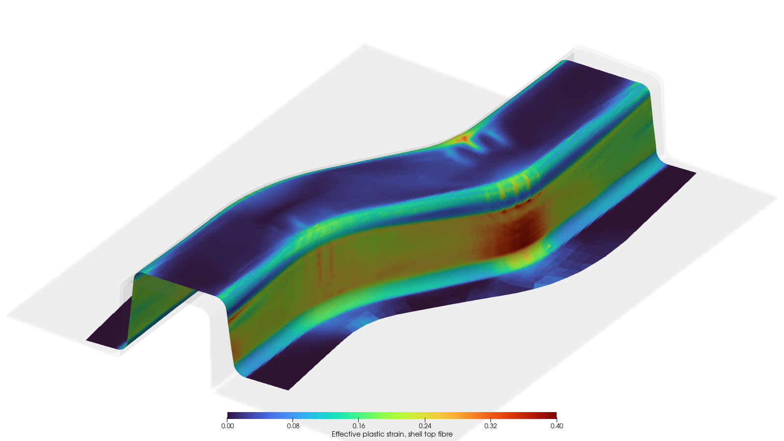
Follow a sheet as it is drawn into an S-shaped rail. Color shows effective plastic strain at the shell top fibre.
Capability demonstration. The animation shows the evolving mesh; the hero image shows the result without mesh lines. This is separate from the runtime case below.
Open videoThese clips demonstrate configured capabilities. Independent numerical validation is documented separately. See validation scope ↗
02 / The value of shorter runtimes
Make room for the next design iteration. This solid-compression scenario shows how the CPU comparison basis changes the runtime ratio.
Illustrative CPU-to-GPU runtime ratio
Supplied timing assumptions · one configurationFP32 GPU / extended-single CPU configuration on separate EPYC 9274F-class servers. Time increments and output differ. Final-field equivalence is not established for this timing case. *Increment count comes from the corresponding completed GPU run.
Read the assumptions and observed runtimesA scenario for one model, not a product-wide speed guarantee. The observed 8-thread CPU and GPU full-run times are available alongside the projections.
One NVIDIA L40 versus Solver B. Compare the same problem families with 8 CPU threads and 1 CPU thread.
A sheet stretches over a rounded punch.
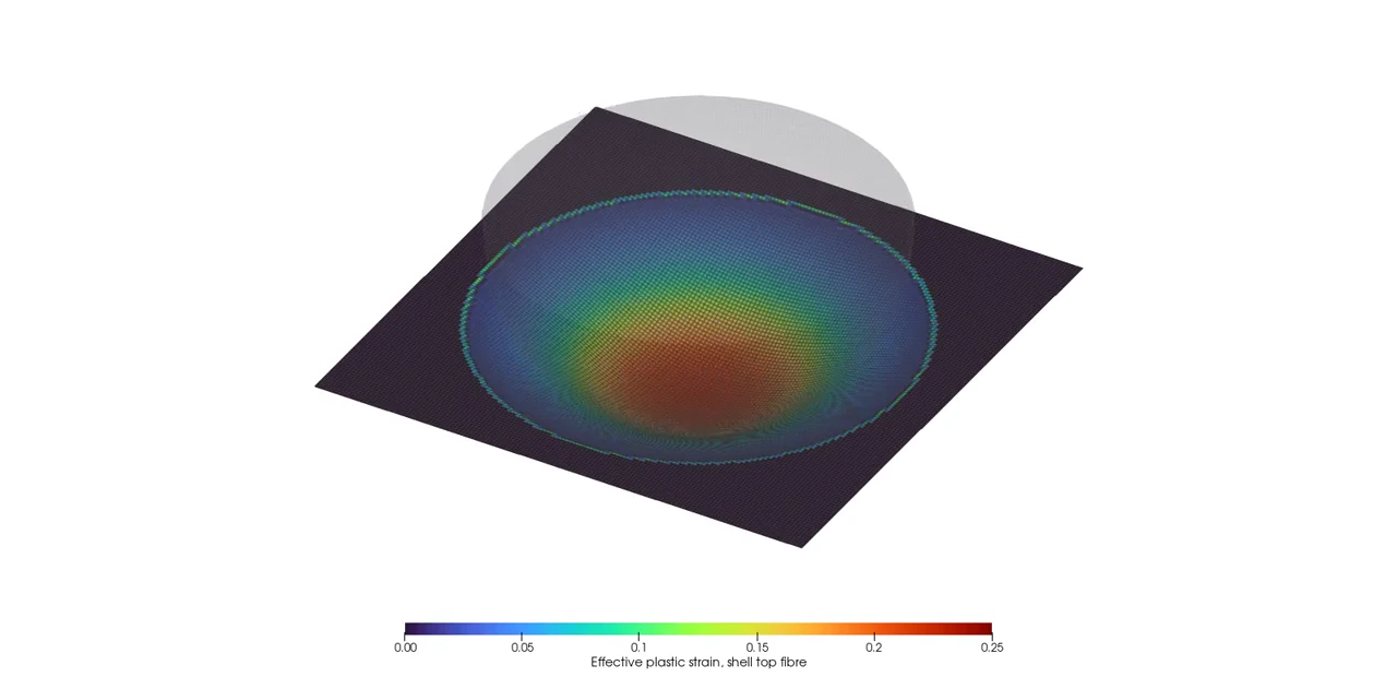
Representative result · 19,881 elements
Shell and solid specimens bend under tooling.
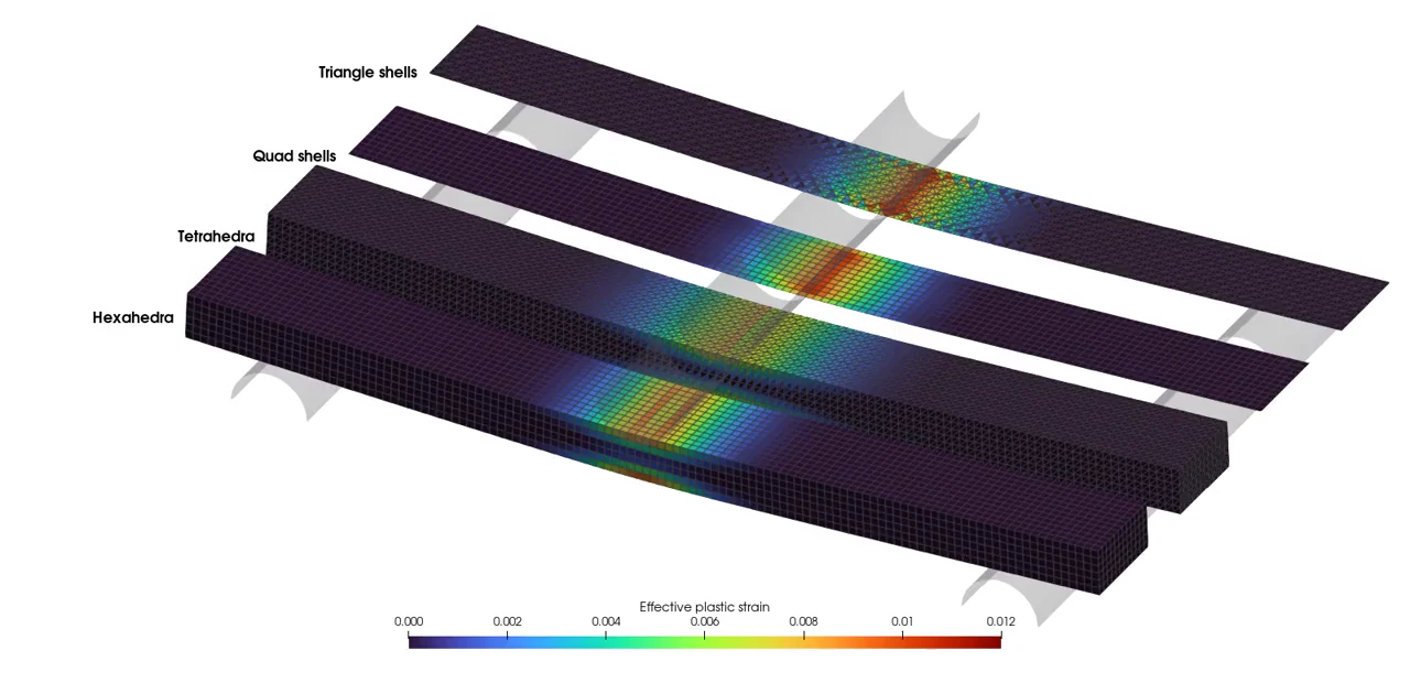
Contact illustration · timing series: no contact
A rigid hemisphere presses into a solid block.
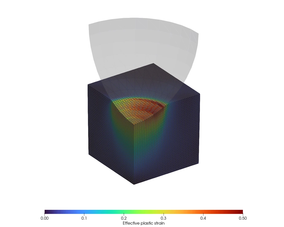
Representative result · 384,000 elements
Match each model title’s color to its curve below. Images show representative results; the curves cover multiple model sizes.
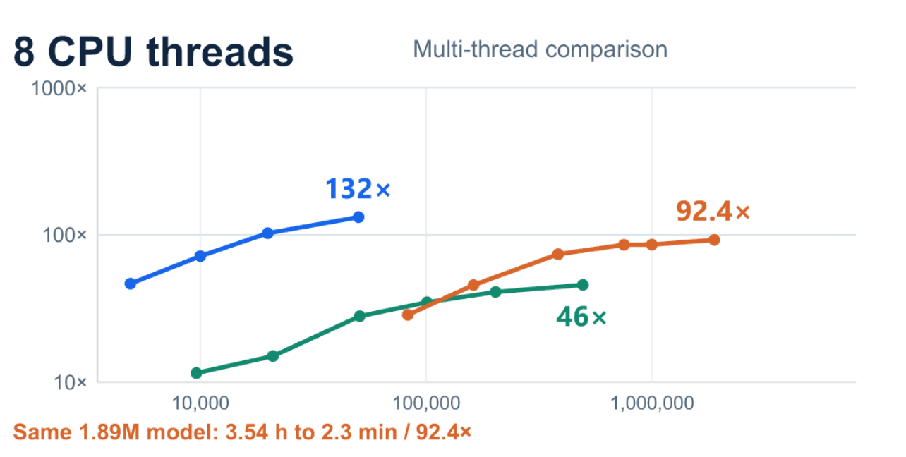
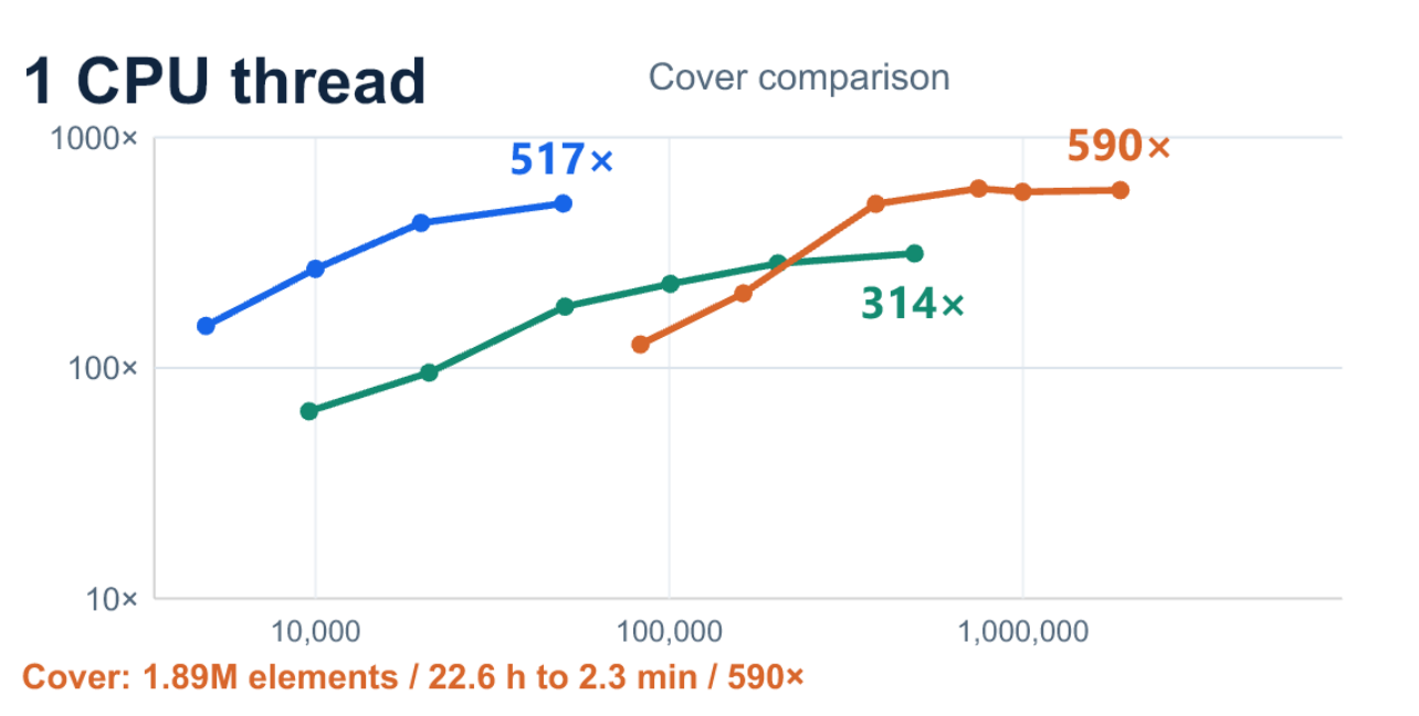
X: element count. Y: CPU time / GPU time. Both panels use the same logarithmic axes.
Illustrative scenarios using supplied timing assumptions, including recorded timings and estimates. Endpoint labels refer to the largest plotted model in each family. Bending timing uses prescribed motion without contact; the gallery shows separate contact examples. Comparison conditions and data ↗
03 / Physics data for AI
Representative physics data is part of the foundation for surrogate models. Faster simulation can change the cost of exploring that data space.
Multiply a recorded single-run time by a chosen number of sequential simulations.
MeshGraphNets used 1,000 training trajectories per dataset. It is an example of dataset scale, not a universal requirement. Read the study ↗
Per run: CPU 6,839.55 s · GPU 66.676 s
Per run: CPU 1,429.374 s · GPU 226.817 s
Both charts share a linear scale. CPU: Solver B on 8 EPYC 9274F threads. GPU: one NVIDIA L40. Single-precision configurations.
Illustrative arithmetic, not measured sustained throughput or a completed dataset. Sequential runs on one CPU allocation or one GPU; concurrent CPU jobs would change the comparison. Data preparation and AI model training time are excluded. Scenario details ↗
The hardware opportunity
Selected hardware generations show how compute and memory bandwidth have developed. This creates room to explore larger models and more physics data for AI.
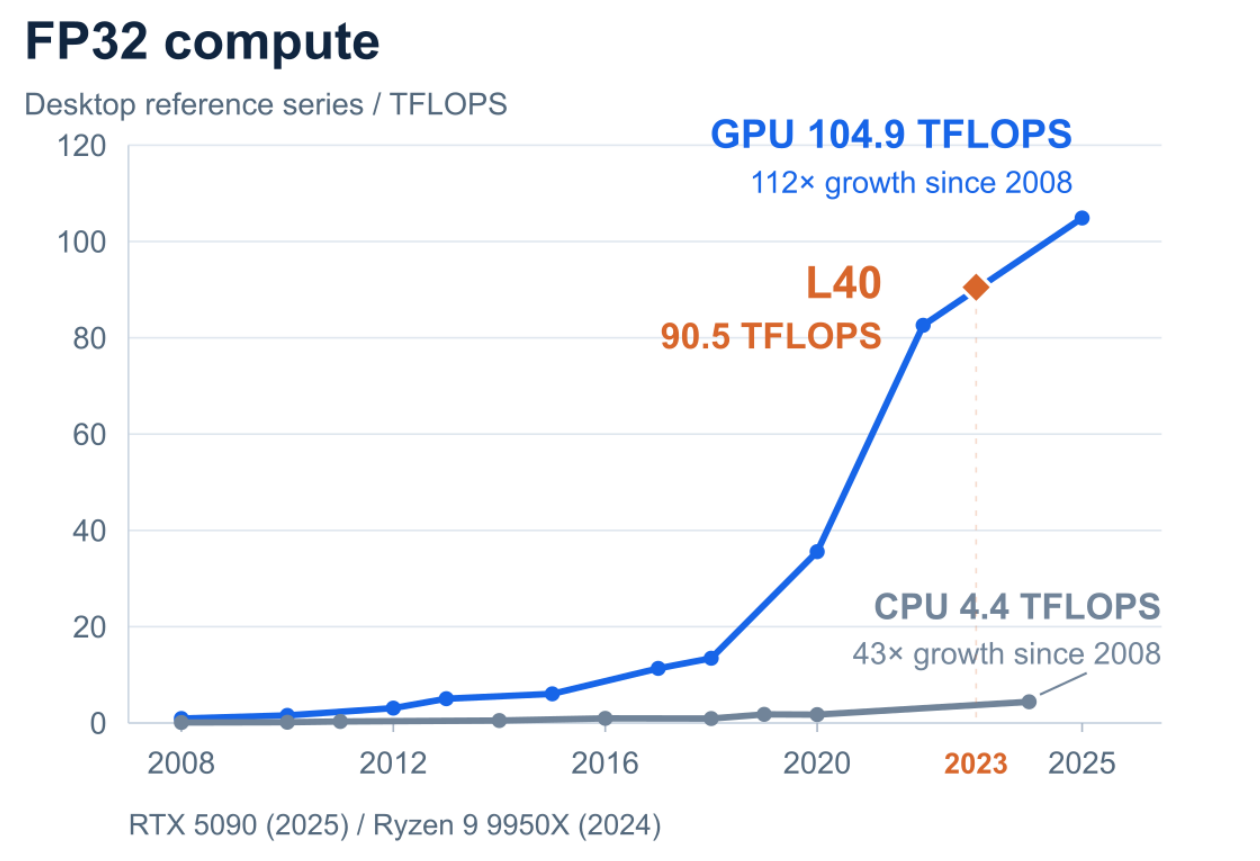
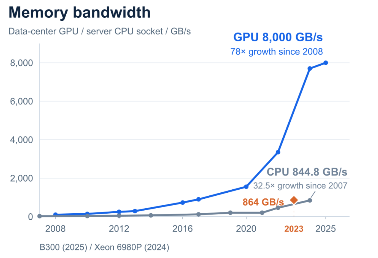
The MinuteSim comparisons on this page use NVIDIA L40.
SUPPORTED hardware specifications. Absolute linear axes. GPU values follow published FP32 conventions; CPU compute values are theoretical at base clocks. Growth labels use each series’ own starting value. B300 bandwidth is up to 8,000 GB/s for the selected configuration. The L40 marker uses 2023 OVX system availability. These specifications do not predict solver speed or compare matched price and power. Products, conventions and sources ↗
Historical source data: Karl Rupp, CPU, GPU and MIC Hardware Characteristics over Time, CC BY 4.0, and Epoch AI, Data on machine learning hardware (CC BY 4.0), plus selected vendor specifications. Figures redrawn with absolute axes and an added L40 reference; graph extracts from the v11 presentation.
04 / The solver today
Supported combinations vary by element, material, contact and constraint. Availability in the documented beta is narrower.
05 / Evidence you can follow
Selected shell, forming and normal-contact configurations have independent numerical validation. Explore the methods, results and limitations.
Canonical verification, Nakajima forming validation against Abaqus/Explicit, and scoped throughput benchmarking.
VALIDATED · specified configurationsJMMP · 2026 ↗Published solid-element studies, scaling, precision comparisons and normal-contact validation.
VALIDATED · specified configurationsLet’s explore the fit
Discuss a representative workload, the results that matter, and a technical evaluation under agreed conditions.
FOR CAE TECHNOLOGY & PRODUCT TEAMS